Quantile Estimation in Distributed Datasets

Introduction

This article summarizes my work and research on quantile estimation for analyzing user behavior across multiple platforms while preserving privacy.

I will present an intuitive, step-by-step method for estimating quantiles in distributed datasets without the need to centralize data. The approach starts with simple averaging, progresses to weighted averages, and culminates in advanced techniques. I will introduce a novel application of the Hölder mean, which enhances the accuracy of estimating extreme quantiles (0th and 100th percentiles) in distributed datasets.

In addition, I will explore the mathematical foundations of each method, including links to U-statistics, the law of total probability, and conditional Monte Carlo methods. This article aims to provide insights into the intersection of privacy-preserving analytics and advanced statistical techniques.

Problem Statement

Imagine a tech company trying to understand user engagement across different platforms without compromising user privacy. Each platform collects data on daily active minutes per user, but we can’t centralize this sensitive information.

Quantiles offer a holistic way to describe user engagement. They tell us, for example, that 75% of users are active for less than 70 minutes a day, or that 25% of users are active for more than 70 minutes a day.

Our goal is to estimate these quantiles for the global dataset without centralizing the data. Key challenges include:

1) Preserving user privacy

2) Handling different sample sizes among platforms

3) Dealing with potential outliers

4) Ensuring computational efficiency in a distributed setting

Chapter 1: Intuition based approach

Metrics

Although error percentages offer intuitive interpretability for comparing various methodologies, the Mean Squared Error (MSE) remains a widely accepted and statistically robust metric.

$MSE = \frac{1}{n} \sum_{i=1}^n (\hat{y}_i - y_i)^2$

Where $\hat{y}_i$ is the estimated value, $y_i$ is the true value, and $n$ is the number of observations.

Step 1: Averaging Quantiles

Our initial approach involved a straightforward averaging of quantiles from each platform. For estimating the p-th quantile, we employed the following formula:

$Q_{avg}(p) = \frac{1}{M} \sum_{j=1}^M Q_j(p)$

Where:

$Q_{avg}(p)$ is the estimated p-th quantile

$Q_j(p)$ represents the p-th quantile from platform j

$M$ denotes the total number of platforms

This method, while intuitive, serves as a baseline for comparison with more sophisticated techniques.

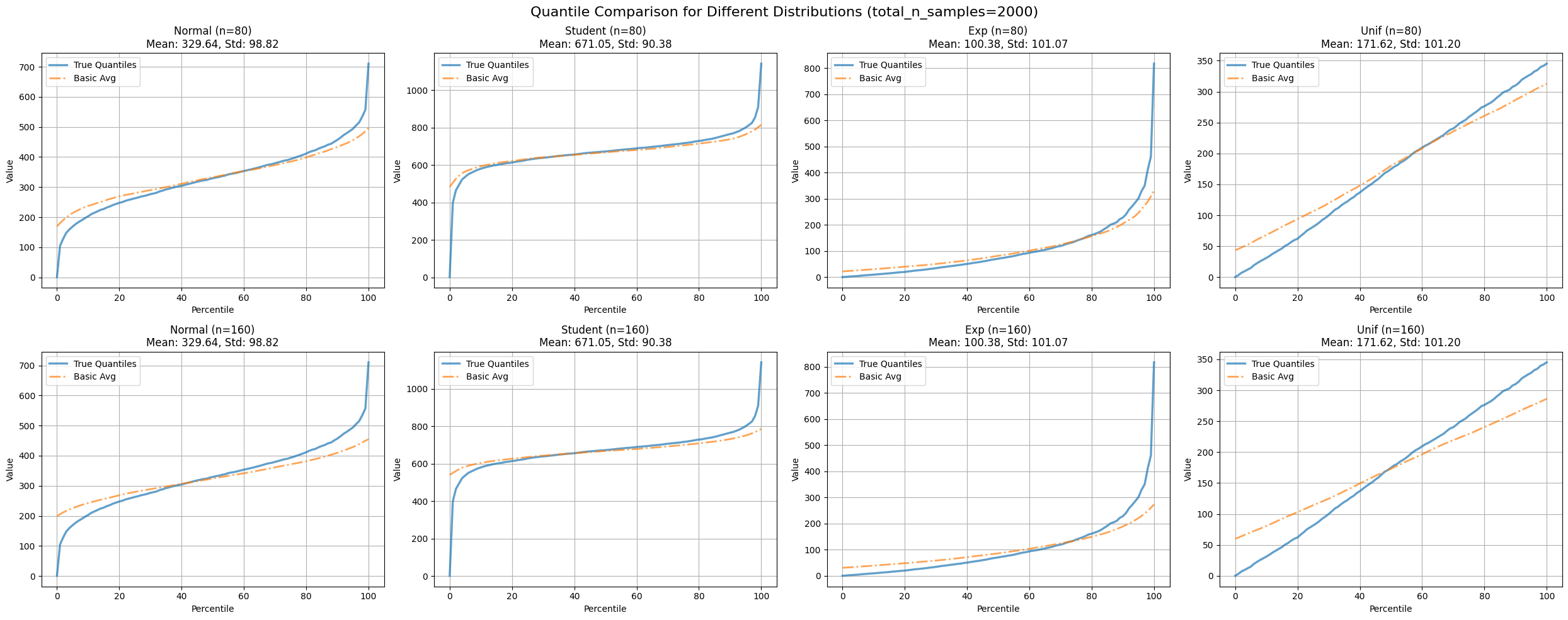
Figure 1: Compares average quantile estimates with true quantiles across various distributions and partition numbers.

distribution	n_partitions	mse_avg
exp	80	3109.81
	160	4452.37
normal	80	1297.89
	160	2245.04
student	80	3890.41
	160	5164.50
unif	80	107.26
	160	260.13

Table 1: MSE comparison between average quantile estimates and true quantiles for different distributions and partition counts.

This approach combines information from all platforms, which intuitively seems like a step in the right direction. However, it presents several significant limitations:

1) Sensitivity to outliers

2) Disregard for varying sample sizes among platforms

3) Assumption of equal representativeness across platforms

To illustrate these weaknesses, consider the following example:

Imagine we have three platforms:

1) MobileApp: 1000 users, 75th percentile at 90 minutes

2) WebApp: 1000 users, 75th percentile at 80 minutes

3) SmartTVApp: 10 users, 75th percentile at 240 minutes

Using simple averaging, the estimated 75th percentile would be:

$(90 + 80 + 240) / 3 = 136.67 \text{ minutes}$

This calculation significantly overestimates the true 75th percentile for the vast majority of users due to the outlier from the SmartTVApp with its small sample size. Ideally, we would want a method to modulate a partition’s contribution based on its sample size, thereby mitigating the impact of outliers from smaller datasets.

Step 2: Weighted Averaging - Giving Credit Where It’s Due

To address the issues with simple averaging, particularly the sample size problem, we implemented a weighted average approach:

$Q_{weighted}(p) = \frac{\sum_{j=1}^M w_j \cdot Q_j(p)}{\sum_{j=1}^M w_j}$

Where:

$Q_{weighted}(p)$ is the weighted estimate of the p-th quantile

$w_j$ is the weight based on sample size for each platform’s quantile estimate

$Q_j(p)$ represents the p-th quantile from platform j

$M$ denotes the total number of platforms

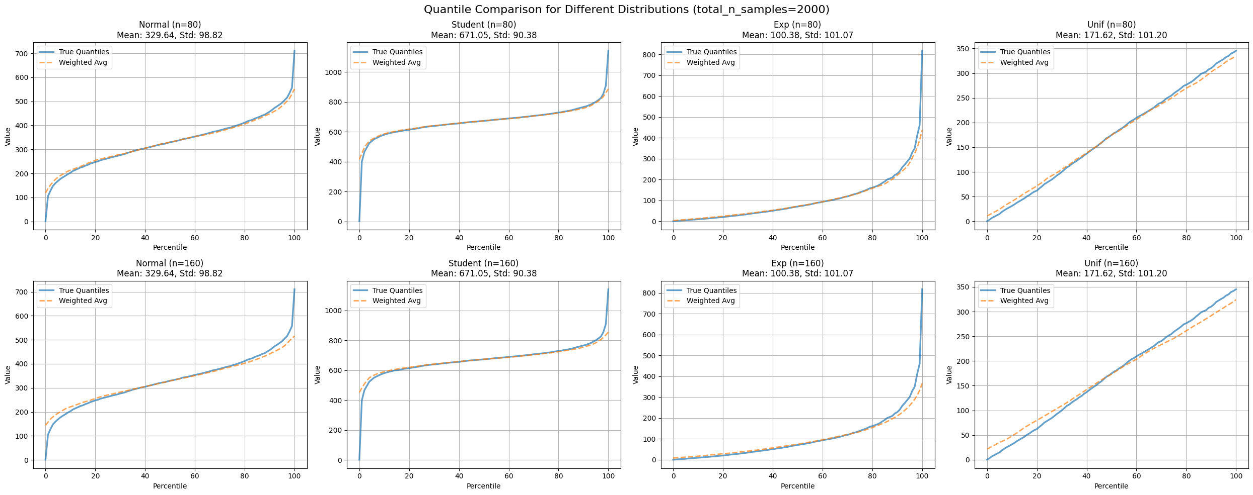
Figure 2: Compares weighted average quantile estimates with true quantiles across various distributions and partition numbers.

distribution	n_partitions	mse_weighted_avg
exp	80	1556.059983
	160	2453.986383
normal	80	457.000396
	160	791.888180
student	80	2428.886730
	160	3040.792046
unif	80	9.693968
	160	38.546067

Table 2: MSE comparison between weighted average quantile estimates and true quantiles for different distributions and partition counts.

This approach gives more weight to platforms with larger sample sizes, which intuitively makes sense - we should place greater trust in data from platforms that have observed more users.

Revisiting our previous example:

1) MobileApp: 1000 users, 75th percentile at 90 minutes

2) WebApp: 1000 users, 75th percentile at 80 minutes

3) SmartTVApp: 10 users, 75th percentile at 240 minutes

Using simple averaging, the estimated 75th percentile was:

$(90 + 80 + 240) / 3 = 136.67 \text{ minutes}$

With weighted averaging (weights proportional to sample size), we get:

$\frac{(90 \cdot 1000 + 80 \cdot 1000 + 240 \cdot 10)}{(1000 + 1000 + 10)} = 85.25 \text{ minutes}$

Step 3: Enter the Hölder Mean - A Mathematical Journey

While the weighted average improved our estimates, we still faced challenges at the very beginning and end of our quantile range (the minimum and maximum values). Even weighted averaging falls short in these extreme cases.

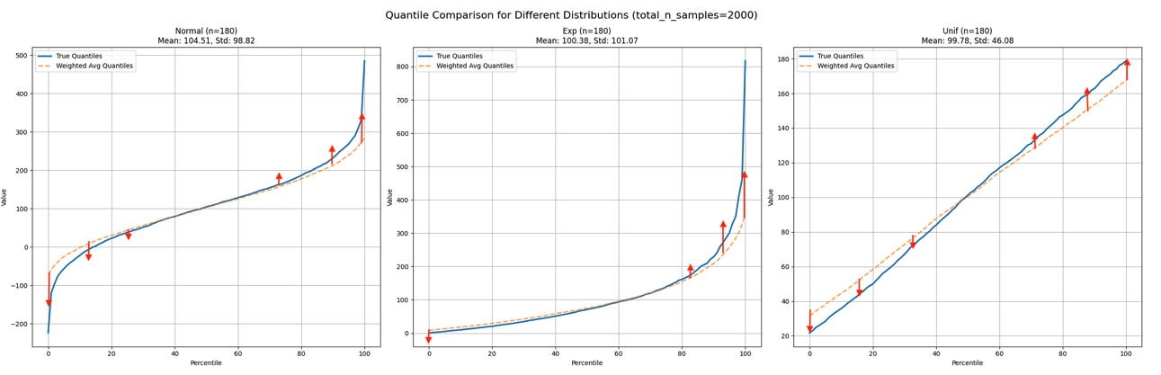
Figure 3: Illustrates desired behavior near 0th and 100th percentiles.

It appears we need to adjust the extremities at a certain rate, with the highest adjustment at the extremities (0th percentile and 100th percentile) and the lowest around the median.

Why? Let’s examine an example. Imagine three platforms report these maximum daily active times:

1) Platform A: 180 minutes

2) Platform B: 150 minutes

3) Platform C: 165 minutes

A weighted average might give us 165 minutes. However, the true maximum is clearly 180 minutes! We need the actual maximum, not an average of maximums. Similarly, for the minimum, we need the smallest value, not an average of small values.

The challenge lies in that we can’t simply use the min and max functions. We require a smooth transition from minimum to average to maximum as we move through our quantile range.

This is where our accidental rediscovery comes into play. We needed a function that could smoothly transition from minimum to average to maximum. Here’s how we stumbled upon it:

To obtain the maximum, we considered: “What if we raised each number to a very high power before averaging?” The largest number would dominate.

For a list $[x_1, x_2, ..., x_n]$ , we derived:

$H_r(x_1, ..., x_n) = (\frac{1}{n}\sum_{i=1}^n x_i^r)^{\frac{1}{r}}$

This function exhibits the following properties:

1) As $r$ approaches infinity, it yields the maximum.

2) When $r = 1$ , it equates to the arithmetic mean.

3) As $r$ approaches negative infinity, it produces the minimum.

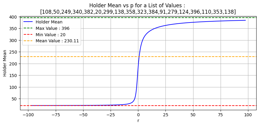
Figure 4: Demonstrates Hölder mean effect on positive integers for varying r values.

It turns out this tool exists already , known as Hölder mean or generalised mean or power mean [1] . You might notice resemblance with p-norm expression if we remove the division by N.

We extended the Hölder Mean by introducing weights:

$H_p(x_1, ..., x_n; w_1, ..., w_n) = \left(\frac{\sum_{i=1}^n w_i \cdot x_i^p}{\sum_{i=1}^n w_i}\right)^{\frac{1}{p}}$

$Q_{holder}(p) = H_r(Q_1(p), ..., Q_M(p); w_1, ..., w_M)$

Where $r$ is our parameter that varies based on the position in the quantile range. Near the edges (0th and 100th percentiles), we push $r$ towards $\pm\infty$ to capture true minimums and maximums. In the middle, we keep it close to 1 for a weighted average behavior.

For $r = 0$ , the Hölder mean becomes the geometric mean.

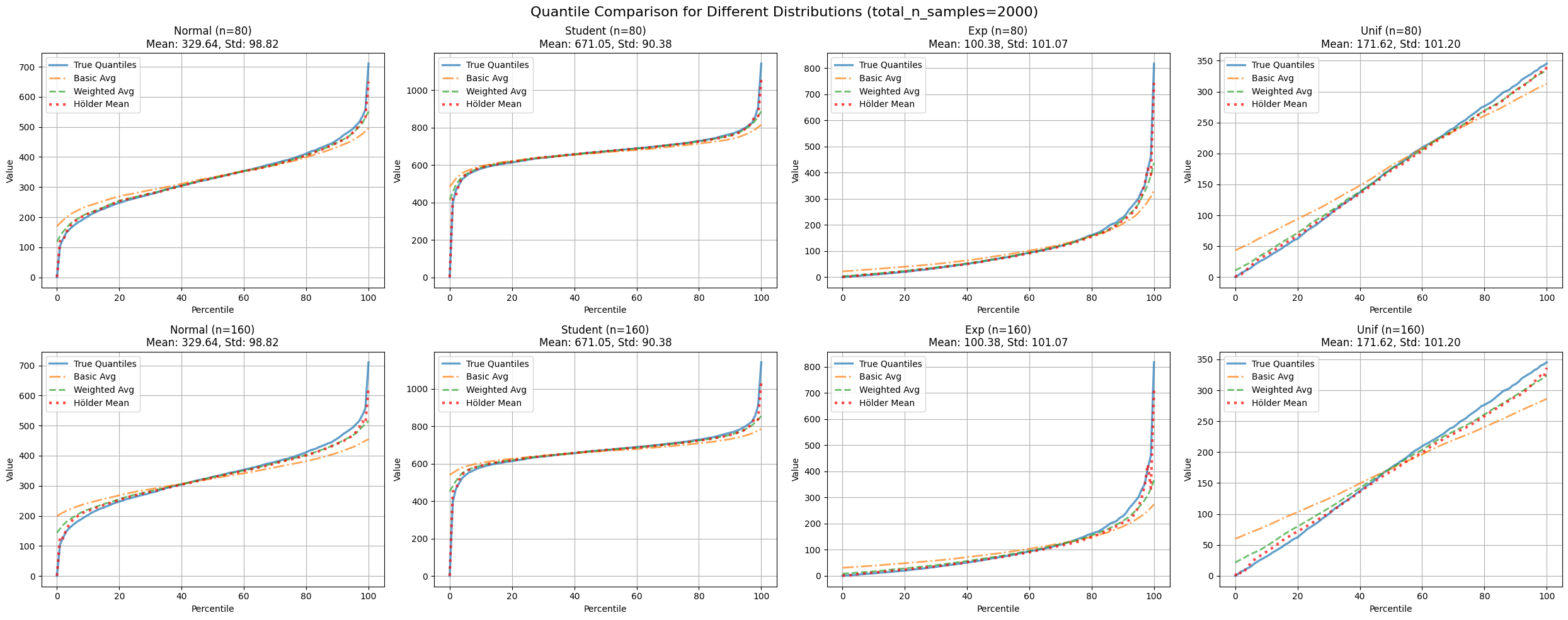
Figure 5: Compares Hölder mean-adjusted weighted average quantile estimates with true quantiles across distributions and partition numbers.

distribution	n_partitions	mse_avg	mse_basic_avg	mse_holder
exp	80	1556.05	3109.81	146.24
	160	2453.98	4452.37	417.82
normal	80	457.00	1297.89	78.93
	160	791.88	2245.04	201.41
student	80	2428.88	3890.41	124.94
	160	3040.79	5164.50	233.32
unif	80	46.75	517.36	32.28
	160	185.91	1254.64	134.93

Table 3: MSE comparison for Hölder mean-adjusted weighted average quantile estimates.

This method accurately captures those challenging minimum and maximum values while maintaining fidelity to the weighted average in the middle range. The figure above illustrates how our method compares to simpler approaches. The choice of r is crucial and can be optimized based on the specific characteristics of your data and the desired balance between averaging and extreme value preservation.

Chapter 2: Mathematical Framework

Let’s see how consistent this is from a theoretical point of view

Metrics: Pinball loss

MSE has served us well so far. However, during my research into similar problems, I discovered a new metric: the pinball loss.

$L_\tau(y,\hat{y})=\max(\tau(y-\hat{y}),(\tau-1)(y-\hat{y}))$

Where $\hat{y}$ is the estimated quantile, $y$ is the true value, and $\tau$ is the quantile level (e.g., 0.5 for median). Pinball loss is advantageous because:

1) It’s specifically designed for quantile regression. 2) It penalizes over-estimation and under-estimation differently. 3) It’s more robust to outliers than MSE. 4) It allows for asymmetric error penalties, useful for many real-world scenarios. 5) It’s convex, making optimization easier.

Let’s examine the previous comparisons using pinball loss:

distribution	n_partitions	mse_avg	mse_basic_avg	mse_holder	pinball_avg	pinball_basic_avg	pinball_holder
exp	80	1556.06	3109.82	146.25	0.73	3.46	0.63
	160	2453.99	4452.38	417.82	1.60	4.87	1.19
normal	80	457.00	1297.90	78.94	0.76	2.38	0.80
	160	791.89	2245.04	201.42	1.18	3.69	1.24
student	80	2428.89	3890.41	124.95	0.46	2.02	0.82
	160	3040.79	5164.51	233.32	0.75	2.60	0.71
unif	80	46.75	517.37	32.29	0.96	3.03	1.07
	160	185.91	1254.65	134.93	1.97	5.01	1.98

Table 4: Compares all methods across distributions and partition numbers using MSE and pinball loss.

Our new metric provides a different perspective, taking into account the dynamics of the quantile function and its purpose.

Step 1: Averaged Quantiles Estimator and U-statistics

While averaging ECDF can be a good estimator, averaging quantiles generally isn’t [2] . Some papers use averaged quantiles [3] , but there’s limited evidence on their quality as estimators (regarding bias, efficiency, and consistency). It’s unclear if there are specific setups (distributions or parameters) where they perform well. Two papers [4] [5] might offer a starting point for investigation. The second one approaches averaged quantiles estimators as U-statistics, showing potential. Unfortunately, neither is publicly available.

Step 2: Weighted Averaged Quantiles

To get this one, I wondered what the problem would look like from a Bayesian point of view:

1) ECDF Definition:

CDF(a) = P(X ≤ a)

2) Bayes’ Theorem with P(X ≤ a):

$P(X \leq a | D_i) \cdot P(D_i) = P(D_i | X \leq a) \cdot P(X \leq a)$

3) Sum over D_i:

$\sum_i P(X \leq a | D_i) \cdot P(D_i) = \sum_i P(D_i | X \leq a) \cdot P(X \leq a)$

4) Factor P(X ≤ a):

$\sum_i P(X \leq a | D_i) \cdot P(D_i) = P(X \leq a) \cdot \sum_i P(D_i | X \leq a)$

5) Summing over all possible events:

$\sum_i P(D_i | X \leq a) = 1$

6) Final Marginal Probability:

$P(X \leq a) = \sum_i P(X \leq a | D_i) \cdot P(D_i)$

Which is the law of total probability. So far, weighted average of ECDF makes sense.

For the next steps we will need these 2 theorems:

1) Quantile as the inverse of Cumulative Distribution Function [6]

Given a continuous and strictly monotonic cumulative distribution function F_X: ℝ → [0, 1] of a random variable X, the quantile function Q: [0, 1] → ℝ maps its input p to a threshold value x such that the probability of X being less than or equal to x is p.

In terms of the distribution function F, the quantile function Q returns the value x such that:

$F_X(x) := Pr(X \leq x) = p$

This can be written as the inverse of the cumulative distribution function (CDF):

$Q(p) = F_X^{-1}(p)$

2) Convergence of Inverses [7]

Theorem. Let $\{f_n\}_{n=1}^{\infty}$ be a sequence of real injective functions defined on $(a, b) \subseteq \bigcap_{n=1}^{\infty} \text{Dom } f_n$ . If the sequence converges uniformly to a function $f_0$ on this interval, and if $f_0$ is a continuous injection on (a, b) and $(a, \beta) \subseteq \bigcap_{n=1}^{\infty} f_n^{-1}((a, b))$ , then $f_n^{-1}$ converges uniformly to $f_0^{-1}$ on (a, β).

If we suppose the necessary assumptions hold (with possibly some level of abuse of assumptions), and given a discrete probability space:

1) $\sum \text{ECDF}_{D_i} \cdot P(D_i) \to \text{ECDF}$

2) Applying the inverse function (quantile function) to the weighted sum of ECDFs:

$f^{-1}\left(\sum \text{ECDF}_{D_i} \cdot P(D_i)\right) = Q$

3) However, given the non linearity of the quantile function, this does not equal the weighted sum of quantiles:

$f^{-1}\left(\sum \text{ECDF}_{D_i} \cdot P(D_i)\right) \neq \sum Q_{D_i} \cdot P(D_i)$

We can just stop at everaging the ECFFs then inverting to obtain quantiles .One problem arises is the need for a common set of points where ECDFs are evaluated .

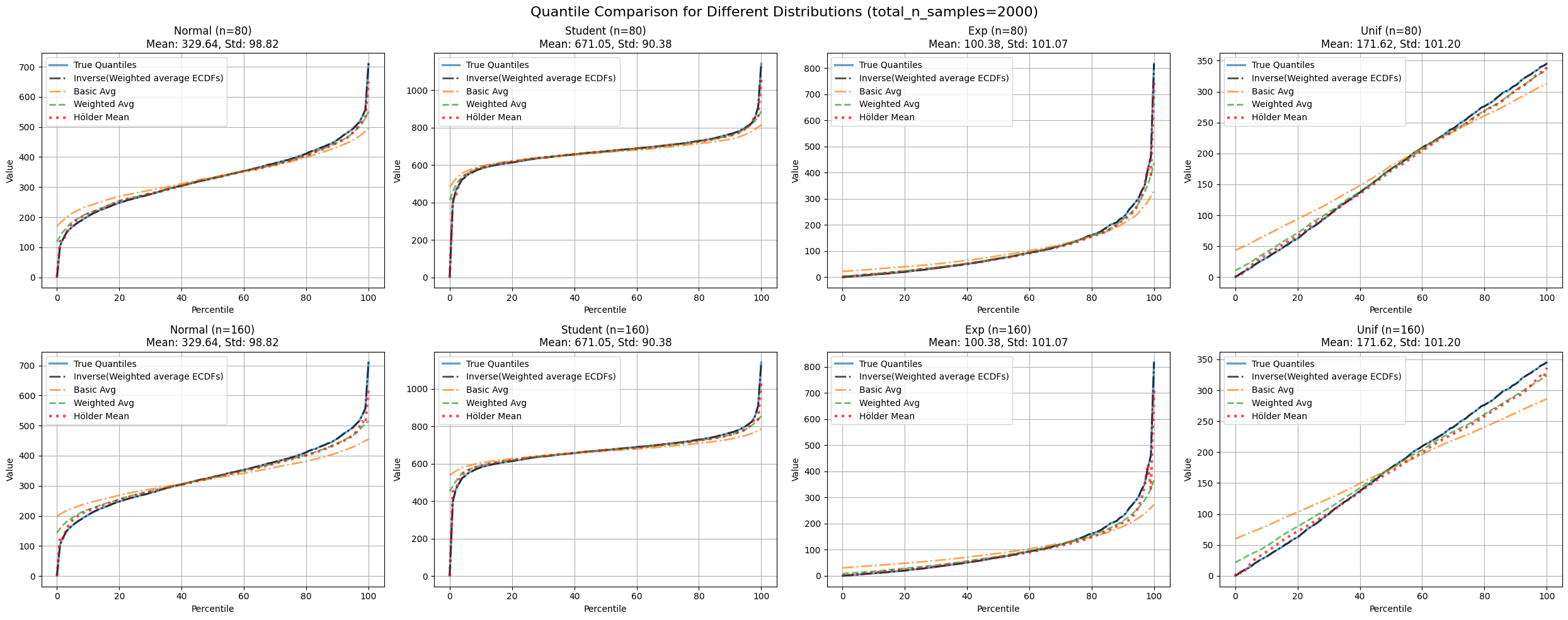
Figure 6: Compares inverse of weighted average ECDF estimate with true quantiles across distributions and partition numbers.

distribution	n_partitions	mse_avg	mse_merged	mse_basic_avg	mse_holder	pinball_avg	pinball_merged	pinball_basic_avg	pinball_holder
exp	80	1556.05	0.003	3109.81	146.24	0.73	0.019	3.45	0.63
	160	2453.98	0.003	4452.37	417.82	1.60	0.019	4.87	1.18
normal	80	457.00	0.051	1297.89	78.93	0.75	0.089	2.37	0.79
	160	791.88	0.051	2245.04	201.41	1.18	0.089	3.68	1.23
student	80	2428.88	0.232	3890.41	124.94	0.45	0.132	2.01	0.82
	160	3040.79	0.232	5164.50	233.32	0.74	0.132	2.59	0.71
unif	80	46.75	0.012	517.36	32.28	0.95	0.047	3.02	1.07
	160	185.91	0.012	1254.64	134.93	1.96	0.047	5.00	1.97

Table 5: Compares all discussed methods (average, weighted average, Hölder mean-adjusted weighted average, inverse of weighted average ECDF) using MSE and pinball loss.

The last two concerns are partly addressed in this paper[8] . They call weighted averaged quantiles “Conditioned Monte Carlo estimator of the quantiles”, and then introduce:

1 Quasi-Monte Carlo (QMC): QMC replaces the n independent random points U_i by a set P_n of n deterministic points u_i = (u_i,1, u_i,2, …, u_i,d) ∈ [0,1)^d which cover the unit hypercube more evenly than typical independent random points. This is done in the sense that their empirical distribution has a low discrepancy with respect to the uniform distribution over [0,1)^d, lower than for typical independent random points.

2 Randomised Quasi-Monte Carlo (RQMC): RQMC turns QMC into a variance reduction method by randomizing the points in a way that they retain their low discrepancy as a group, while each individual point has the uniform distribution over the unit hypercube.

Conclusion

The journey was quite insightful. I got to learn few other things in the process like :

1 t-digest: A data structure for estimating quantiles on streaming data. It’s memory-efficient and handles large data volumes by maintaining a compressed representation of the distribution.[9]

2 Average of quantiles as mean estimator: Quantiles can be viewed as representative samples of a distribution. Averaging these quantiles often provides a good approximation of the distribution’s mean.[10]

3 Value at Risk (VaR): A financial risk measure. It estimates the maximum potential loss in value of a portfolio over a defined period for a given confidence interval. Commonly used in finance for risk management and regulatory reporting.[11]

Besides the valuable insights gained from exploring different techniques, my key takeaway—given the inherent limitations of each approach, such as sensitivity to outliers, computational overhead, and data heterogeneity—is to prioritize aggregating ECDFs instead of quantiles directly.

References

[1] https://en.wikipedia.org/wiki/Generalized_mean

[2] https://doi.org/10.1002/ffo2.139

[3] https://www1.coe.neu.edu/~wxie/A%20pooled%20percentile%20estimator%20for%20parallel%20simulations_2020.pdf

[4] Asymptotic representations for importance-sampling estimators of value-at-risk and conditional value-at-risk Lihua Sun ,L. Jeff Hong

[5] A generalized quantile estimator W.D. Kalgh &Peter A. Lachenbruch

[6] https://en.wikipedia.org/wiki/Quantile_function

[7] https://dml.cz/bitstream/handle/10338.dmlcz/107422/ArchMath_027-1991-2_9.pdf

[8] https://inria.hal.science/hal-02551516/document

[9] https://www.gresearch.com/news/approximate-percentiles-with-t-digests/

[10] https://en.wikipedia.org/wiki/Inverse_transform_sampling

[11] https://www.investopedia.com/terms/v/var.asp